Validation Analysis Help
The validation analysis pages provide information about EM volumes released in EMDB. The information is provided as a set of images and graphs; the exact content depends on what information is available for an entry.
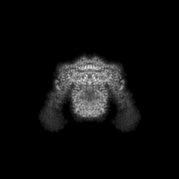
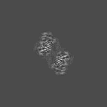
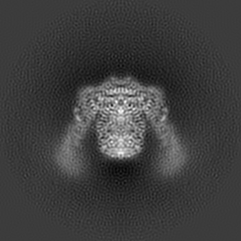
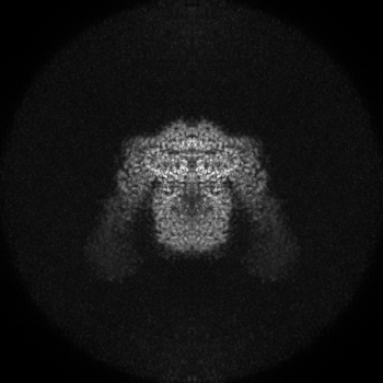
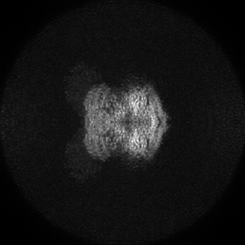
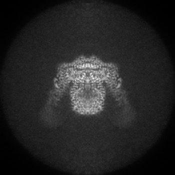
Orthogonal projections
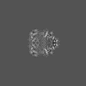
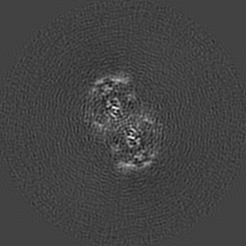
Orthogonal projections are produced for all entries. Images are in grayscale and 300 x 300 pixels in size. Clicking on an image will open a version in it's original size, which may be larger or smaller than the 300x300 pixels. The images show the projection of the map in three orthogonal directions(along the X, Y and Z axes, respectively). The example here is for EMD-0132.
X
Y

Z
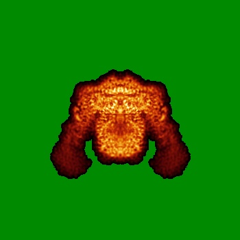
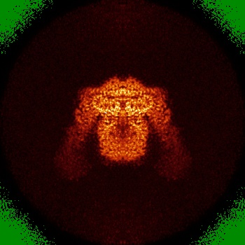
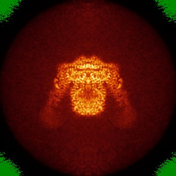
Orthogonal projections (false-colour)
Orthogonal projections with false-colour are produced for all entries. The grey scale
images are match to a color by using color lookup table GLOW (From fiji ).
The minimum value of the projection is match to green with RGB (0, 138, 0) and the maximum value is
match to blue with RGB (0, 0, 255). Any other values will be match to colours between green and blue
as this colour bar (  ).
Images are 300 x 300 pixels in size.
Clicking on an image will open a version in it's original size,
which may be larger or smaller than the 300x300 pixels.
The images show the projection of the map in three orthogonal directions (along the X, Y and Z axes,
respectively).
The example here is for EMD-0132.
).
Images are 300 x 300 pixels in size.
Clicking on an image will open a version in it's original size,
which may be larger or smaller than the 300x300 pixels.
The images show the projection of the map in three orthogonal directions (along the X, Y and Z axes,
respectively).
The example here is for EMD-0132.

X

Y

Z
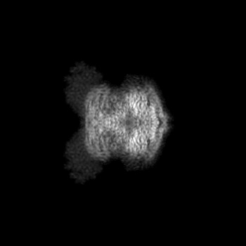
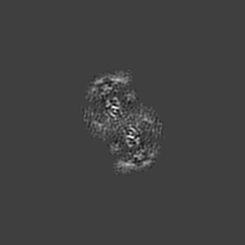
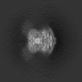
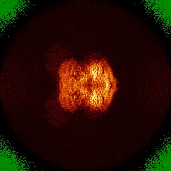
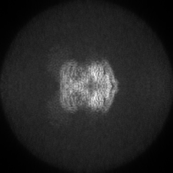
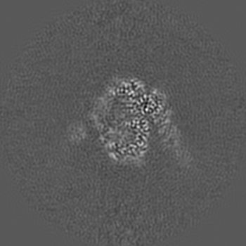
Orthogonal maximum-value projections
Orthogonal maximum-value projections are produced for all entries. Each pixel in the image is the maximum value along that dimension. Images are in grayscale and 300 x 300 pixels in size. Clicking on an image will open a version in it's original size, which may be larger or smaller than the 300x300 pixels. The images show the projection of the map in three orthogonal directions(along the X, Y and Z axes, respectively). The example here is for EMD-0132.
X
Y

Z
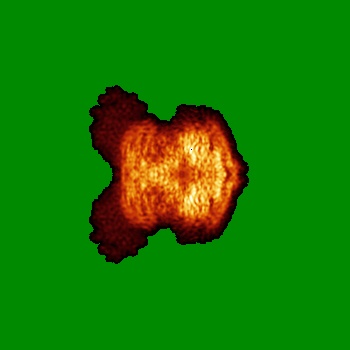
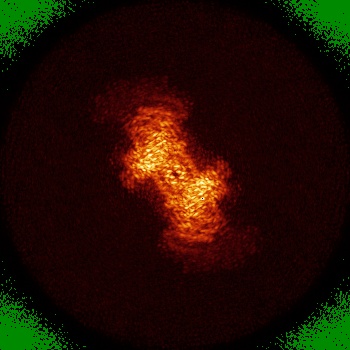
Orthogonal maximum-value projections (false-colour)
Orthogonal maximum-value projections with false-colour are produced for all entries. The grey scale
images are match to a color by using color lookup table GLOW (From fiji ).
The minimum value of the projection is match to green with RGB (0, 138, 0) and the maximum value is
match to blue with RGB (0, 0, 255). Any other values will be match to colours between green and blue
as this colour bar ( ).
Images are 300 x 300 pixels in size.
Clicking on an image will open a version in it's original size,
which may be larger or smaller than the 300x300 pixels.
The images show the projection of the map in three orthogonal directions(along the X, Y and Z axes,
respectively).
The example here is for EMD-0132.

X

Y
Z
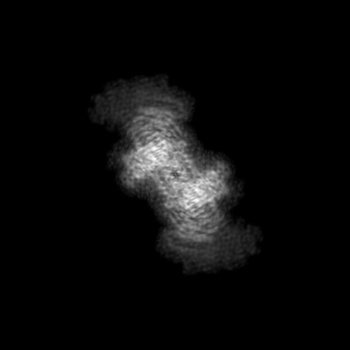
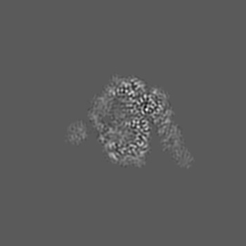
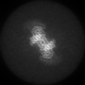
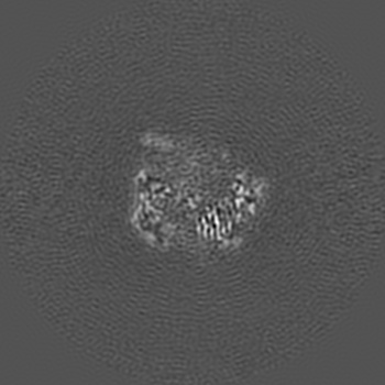
Orthogonal standard-deviation projections
Orthogonal standard-deviation projections are produced for all entries. Each pixel value represents the standard deviation along that corresponding dimension. Images are in grayscale and 300 x 300 pixels in size. Clicking on an image will open a version in it's original size, which may be larger or smaller than the 300x300 pixels. The images show the projection of the map in three orthogonal directions(along the X, Y and Z axes, respectively). The example here is for EMD-0132.
X
Y
Z
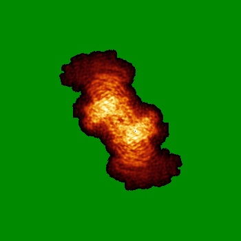
Orthogonal standard-deviation projections (false-colour)
Orthogonal standard-deviation projections with false-colour are produced for all entries. The grey scale
images are match to a color by using color lookup table GLOW
(From fiji).
The minimum value of the projection is match to green with RGB (0, 138, 0) and the maximum value is
match to blue with RGB (0, 0, 255). Any other values will be match to colours between green and blue
as this colour bar ( ).
Images are 300 x 300 pixels in size.
Clicking on an image will open a version in it's original size,
which may be larger or smaller than the 300x300 pixels.
The images show the projection of the map in three orthogonal directions(along the X, Y and Z axes,
respectively).
The example here is for EMD-0132.
X
Y
Z
Central slices
Central slices are provided for tomograms in place of the orthogonal surface projections. Images are in grayscale and 300 x 300 pixels. Clicking on an image will open a version in it's original size, which may be larger or smaller than the 300x300 pixels. The images show the central slice of the map in three orthogonal directions(along the X, Y and Z axes, respectively). The example here is for EMD-0132.
X
Y
Z
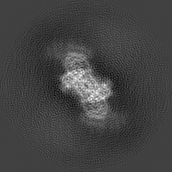
Largest variance slices
Largest variance slices are provided for all entries. Images are 300 x 300 pixels. Clicking on an image will open a version in it's original size, which may be larger or smaller than the 300x300 pixels. The images show the largest variance slices of the map in three orthogonal directions(along the X, Y and Z axes, respectively). The example here is for EMD-0132. These images, especially in the case of tomograms, may point to planes in the map that are "interesting" and have lots of signal and contrast.
X Index: 164
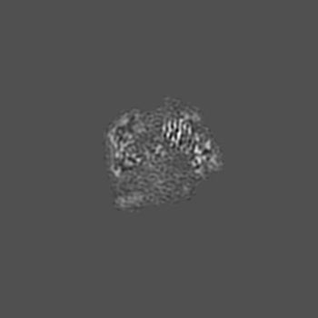
Y Index: 166
Z Index: 192
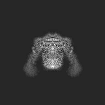
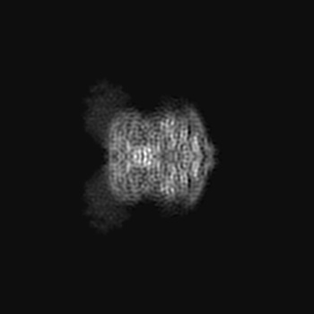
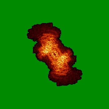
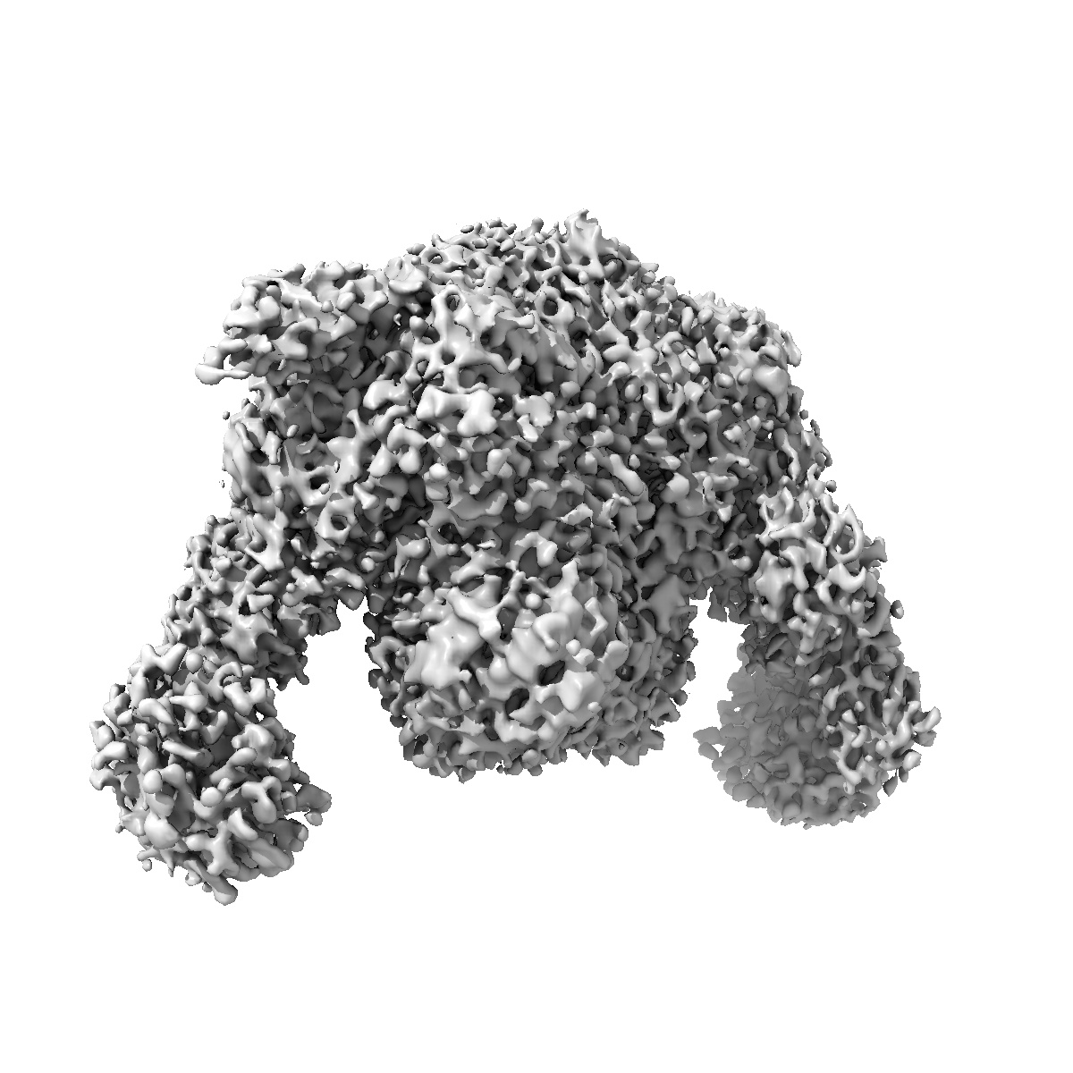
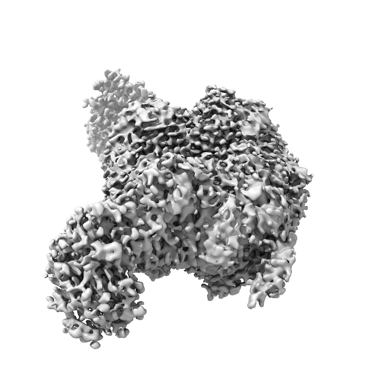
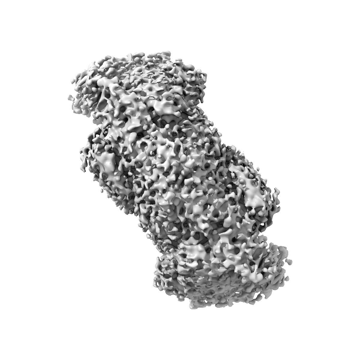
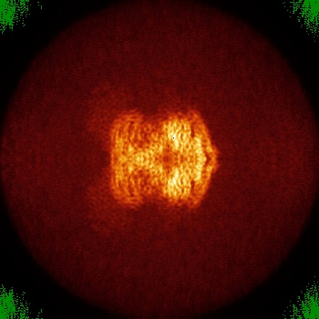
Orthogonal surface views
Orthogonal surface views are provided for non-togomgram entries. Images are 300 x 300 pixels. Clicking on an image will open a larger version, 1200 x 1200 pixels. There are three images, taken along X, Y, and Z, independent of the shape, at the recommended contour level. The provenance of the contour level is also given, and can be author-provided, determined by EMDB staff, or unknown. Some entries do not have a recommended contour level; in these cases the images are contoured at one standard deviation above the average value. The example here is for EMD-0132. The images have been rendered by using ChimeraX.
X
Y
Z
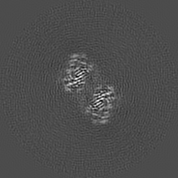
Orthogonal projections of raw map
Orthogonal projections of raw map are produced for all entries. Images are in grayscale and 300 x 300 pixels in size. Clicking on an image will open a version in it's original size, which may be larger or smaller than the 300x300 pixels. The images show the projection of the map in three orthogonal directions(along the X, Y and Z axes, respectively). The example here is for EMD-0132.
X
Y
Z
Orthogonal projections of raw map (false-colour)
Orthogonal projections of raw map with false-colour are produced for all entries.
The minimum value of the projection is match to green with RGB (0, 138, 0) and the maximum value is
match to blue with RGB (0, 0, 255). Any other values will be match to colours between green and blue
as this colour bar ( ).
Images are 300 x 300 pixels in size.
Clicking on an image will open a version in it's original size,
which may be larger or smaller than the 300x300 pixels.
The images show the projection of the map in three orthogonal directions(along the X, Y and Z axes,
respectively).
The example here is for EMD-0132.

X

Y

Z
Orthogonal maximum-value projections of raw map
Orthogonal maximum-value projections of raw map are produced for all entries. Each pixel in the image is the maximum value along that dimension. Images are in grayscale and 300 x 300 pixels in size. Clicking on an image will open a version in it's original size, which may be larger or smaller than the 300x300 pixels. The images show the projection of the map in three orthogonal directions(along the X, Y and Z axes, respectively). The example here is for EMD-0132.
X
Y

Z
Orthogonal maximum-value projections of raw map (false-colour)
Orthogonal maximum-value projections of raw map with false-colour are produced for all entries. The grey scale
images are match to a color by using color lookup table GLOW (From fiji ).
The minimum value of the projection is match to green with RGB (0, 138, 0) and the maximum value is
match to blue with RGB (0, 0, 255). Any other values will be match to colours between green and blue
as this colour bar ( ).
Images are 300 x 300 pixels in size.
Clicking on an image will open a version in it's original size,
which may be larger or smaller than the 300x300 pixels.
The images show the projection of the map in three orthogonal directions(along the X, Y and Z axes,
respectively).
The example here is for EMD-0132.
X
Y
Z
Orthogonal standard-deviation projections of raw map
Orthogonal standard-deviation projections of raw map are produced for all entries. Each pixel value represents the standard deviation along that corresponding dimension. Images are in grayscale and 300 x 300 pixels in size. Clicking on an image will open a version in it's original size, which may be larger or smaller than the 300x300 pixels. The images show the projection of the map in three orthogonal directions(along the X, Y and Z axes, respectively). The example here is for EMD-0132.
X
Y
Z
Orthogonal standard-deviation projections of raw map (false-colour)
Orthogonal standard-deviation projections of raw map with false-colour are produced for all entries. The grey scale
images are match to a color by using color lookup table GLOW
(From fiji).
The minimum value of the projection is match to green with RGB (0, 138, 0) and the maximum value is
match to blue with RGB (0, 0, 255). Any other values will be match to colours between green and blue
as this colour bar ( ).
Images are 300 x 300 pixels in size.
Clicking on an image will open a version in it's original size,
which may be larger or smaller than the 300x300 pixels.
The images show the projection of the map in three orthogonal directions(along the X, Y and Z axes,
respectively).
The example here is for EMD-0132.
X
Y
Z
Central slices of raw map
Same idea as central slice here we also provide central slices of raw map. Images are in grayscale and 300 x 300 pixels. Clicking on an image will open a version in it's original size, which may be larger or smaller than the 300x300 pixels. The images show the central slice of the map in three orthogonal directions (along the X, Y and Z axes, respectively). The example here is for EMD-0132.
X
Y
Z
Largest variance slices of raw map
Largest variance slices of raw map are provided for all entries. Images are 300 x 300 pixels. Clicking on an image will open a version in it's original size, which may be larger or smaller than the 300x300 pixels. The images show the largest variance slices of the map in three orthogonal directions (along the X, Y and Z axes, respectively). The example here is for EMD-0132. These images, especially in the case of tomograms, may point to planes in the map that are "interesting" and have lots of signal and contrast.
X Index: 164
Y Index: 184
Z Index: 192
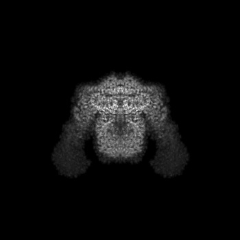
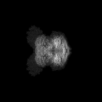
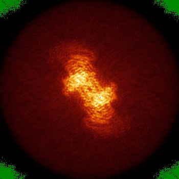
Orthogonal surface views of raw map
Orthogonal surface views of raw map are provided for non-tomogram entries. Images are 300 x 300 pixels. Clicking on an image will open a larger version, 1200 x 1200 pixels. There are three images, taken along X, Y, and Z, independent of the shape, at the recommended contour level. The provenance of the contour level is also given, and can be author-provided, determined by EMDB staff, or unknown. Some entries do not have a recommended contour level; in these cases the images are contoured at one standard deviation above the average value. The example here is for EMD-0132. The images have been rendered by using ChimeraX.
X
Y
Z
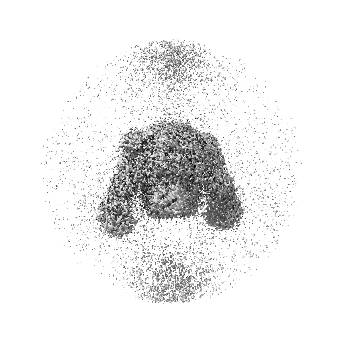
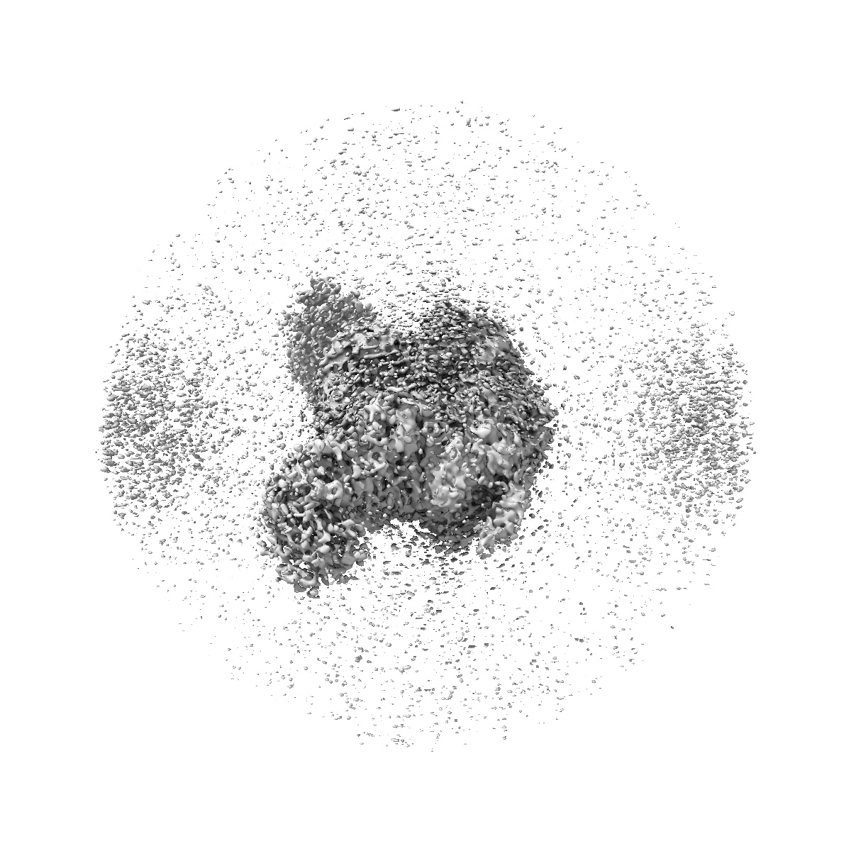
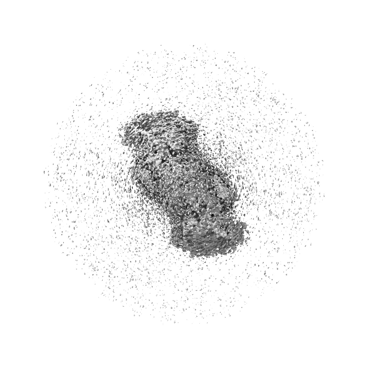
Mask visualisation
Some EMDB entries have one or more masks associated with them. A mask typically either encompasses the whole structure and indicates the removal of noise from the peripheries of the map, or seperates out a domain, a functional unit, a monomer or an area of interest from the larger structure, e.g., EMD-1216. For entries with one or more masks there are three images along X, Y, Z for each mask with the map shown at 50 % opacity, and the provided mask overlaid as an opaque object. In some cases, e.g., EMD-1001, masks were used for subtomogram averages; in such instances the masks do not correspond to any feature in the map, and the images are not likely to provide much insight. The example here is for EMD-0132. The images have been rendered by using ChimeraX.

X

Y

Z
Map-value distribution
For each entry there is a map-value distribution graph, calculated in 128 intervals. The y-axis is logarithmic. A spike in this graph around zero usually indicates that the volume has been masked. EMDB does not yet collect information about masks, and the use of masks are rarely published. Masking is frequently used to remove background noise from an EM volume. This is nothing strange, but the interpretation of the map may be different with knowledge about any masking. The mode value which given as a subtitle. If you see this value is very close to zero, then very likely a mask was applied in the preprocessing procedure of the map. The example here is for EMD-0132.
Volume estimate
The volume-estimate graph shows how the enclosed volume of the map varies with contour level. The specified contour level is shown as a vertical line and the intersection between the line and the curve gives the volume of the enclosed surface at the given threshold. If the molecular weight of the sample is provided by the author, the volume corresponding to the molecular weight is also indicated by a horizontal line. Ideally the horizontal and vertical lines will intersect at a single point on the volume-estimate curve. Volume curve calculation: a density value of 1.5 g/cm³ has been used to provide a rough estimate of the molecular volume, based on the molecular weight. The density of a biological sample can vary to a large degree from as low as 1.2 g/cm³ for some proteins to close to 2 g/cm³ for nucleic acids with CsCl salts. The unit for molecular weight is kDa, and for the volume, nm³. The volume-estimate graph should be treated as tentative. Some reasons why the sample and map-based molecular weights may not agree are:
-
Molecular weight is given for a fraction of the sample, e.g. one repeating unit, when the sample includes many.
-
The weight is given for a larger unit than what is in the EM volume, e.g. a whole fiber.
-
The sample has a greater or smaller than average density.
-
No correction has been made for stained samples.
-
The contour provided by the author may not correspond to the estimated volume.
The example here is for EMD-0132.
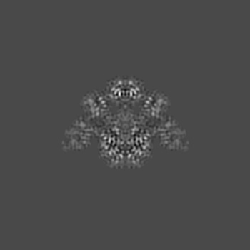
Rotationally averaged power spectrum (RAPS)
For cubic volumes we provide a rotationally averaged power spectrum. The RAPS may provide insight into the processing, in terms of:
-
CTF correction
-
Temperature-factor correction
-
Low and/or high-pass filtering
-
Masking artifacts
The example here is for EMD-0132.
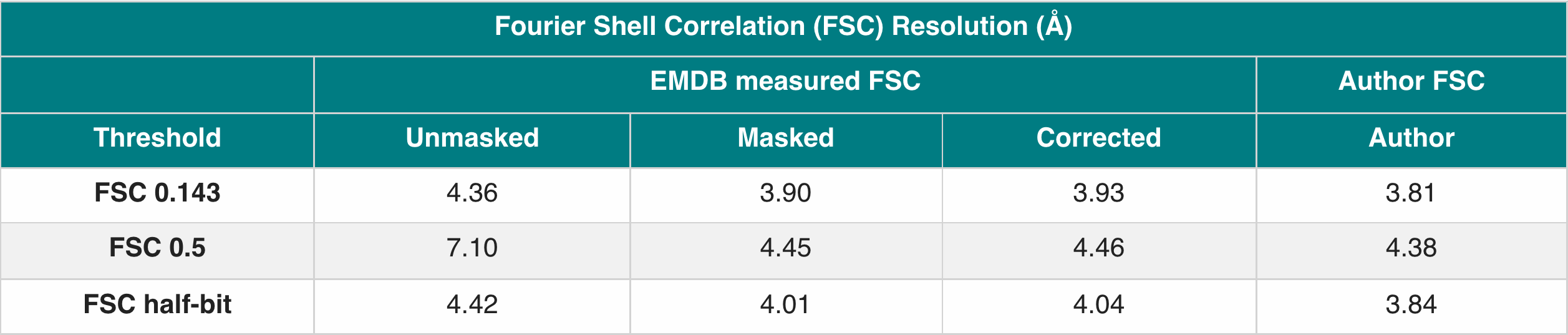
FSC validation
Fourier Shell Correlation (FSC) remains the most widely accepted method for estimating the resolution of single-particle cryo-EM maps archived in EMDB. In the Validation Analysis pipeline, the FSC is calculated using Relion(Scheres, 2012), providing a comparable resolution measurement across entries and for comparison to depositor provided FSC curve data.
What the plot shows
The FSC plot (upper panel) displays the correlation between two independently refined half-maps as a function of spatial frequency.
- Author provided FSC (if provided) — deposited by the submitting laboratory and plotted for reference.
- Author provided resolution Resolution value provided by the author during deposition, shown as a vertical red line.
- Calculated FSC (unmasked, masked, corrected, phase randomization (Chen et al., 2013)) — generated by Relion.
Threshold cut-offs:
- 0.143 FSC cut-off (black dashed line)
- 0.5 FSC cut-off (grey dashed line)
- Half-bit threshold (purple dashed line), representing the information criterion
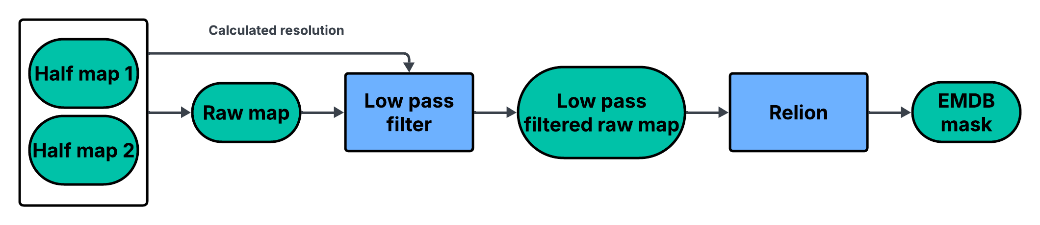
EMDB masks
In the EMDB Validation Analysis pipeline, the EMDB mask is generated using Relion. After combining the depositors two half-maps to form a raw map (Learn more), an initial resolution is estimated from the half-maps (e.g., via unmasked FSC). The raw map is then low-pass filtered using this resolution. Finally, RELION’s mask creation uses the low-passed raw map to produce the EMDB mask(s), with automatic thresholding and a soft edge to avoid mask induced fourier shell correlations.
How to interpret the resolution table
The resolution table (lower panel) summarizes key resolution estimates derived from the FSC curves above.
- Values are reported for unmasked, masked, corrected and phase randomised FSC.
- The author FSC resolution (if deposited) is listed alongside calculated values for direct comparison.
This side-by-side representation provides a comparative global resolution estimation. Where the EMDB mask is successfully generated, the calculated FSC curves may help identify potential overfitting in the map refinement.
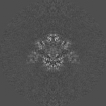
Map-model overlay views
For entries that have one or more fitted models, there is another set of images. For each fitted model there are three images with the model overlayed, taken along X, Y, and Z directions. The maps are drawn at 50 % opacity at the same contour level as used for the map images. Models are drawn as ribbons. The images have been rendered by using ChimeraX. The example here is for EMD-0132

X

Y

Z
Map with assembled model views
For entries that have the symmetry information with the model. Model will be produced with the full assemble and map with full assembled model will be shown. For each fitted model there are three images with the model overlayed, taken along X, Y, and Z directions. The maps are drawn at 50 % opacity at the same contour level as used for the map images. Models are drawn as ribbons. The images have been rendered by using ChimeraX. The example here is for EMD-1011

X

Y

Z
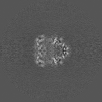
Map-model fit based on residue inclusion
These views show how well the model fits the map based on the all-atom residue-inclusion score. The more red the lower the fractions of atoms that fit the map at recommended contour level. The images have been rendered by using ChimeraX. The example here is for EMD-0132

X

Y

Z
Atom inclusion by residue
Atom inclusion can be calculated as a function of residue. The atom inclusion by residue graph highlights parts of a model that may be outside the map. The calculation is done at the recommended contour level. The result is colour-ramped, with red indicating that a residue is completely outside, and cyan completely inside the map. Each chain starts on a new line, with each line containing up to 200 residues, in the same order as in the model. All atoms are included in the atom inclusion by residue. For models, or parts of models, that only have trace atoms (C-alpha in amino acids/P in nucleic acids), the result is binary, either in or out. For other models, the inclusion value for each is residue is the average for the atoms in that residue. The atom inclusion by residue graph can take some time to load, large models may have up to thousands of residues. In such cases, zooming, saving, and printing will also be slow. The example here is for EMD-0132
Atom inclusion as a function of contour level
For each model fitted in the EM volume an atom-inclusion graph is shown. Models can be trace, backbone, or all atoms, or a combination of these. The atom-inclusion graphs displays the fraction of atoms that are inside the map at a given contour level. For all-atom models, two curves are drawn, one for backbone atoms in blue, and one for all atoms in green. Only in cases where the resolution is sufficiently high to resolve side chains should the all atom graph be used. For some models fitted to modest atom inclusions scores - say 50 % the fitting can look quite good visually. Any information about the protocol for the fitting of the model, e.g., rigid-body, or flexible fitting is currently stored in an optional free text field in the EMDB. The information is included here, it is an aim of the EMDB to make this information more consistent in the future. The example here is for EMD-0132
Map-model FSC
For each model fitted in the EM volume an map-model FSC graph is shown. The FSC is calculated from primary map and the simulated map based on the fitted model. Here simulated map is calculated by using REFMAC5 from CCP4. Map-model FSC resolution is given by user the 0.5 criterion. The example here is for EMD-0132
Q-score distribution
For each model fitted in the EM volume with Q-score result, there Q-socre distribution graph is shown. Models can be trace, backbone, or all atoms, or a combination of these. The Q-score distribution displays the fraction of atoms at its corresponding Q-score level. Q-score values range from -1 to 1 with 100 bins. For all-atom models, two curves are drawn, one for residue in blue, and one for all atoms in green. Well fitted model should have the major part of curve distributed between 0 and 1. In cases where large part of the curve sits in negative range worth further check. The example here is for EMD-0132
Map-model fit based on residue Q-score
These views show how well the model fits the map based on the Q-scores (Grigore et al.). The more red the lower the Q-score is which indicate not well fitted into the map. The images have been rendered by using ChimeraX. The example here is for EMD-0132

X

Y

Z
Q-scores by residue
Q-score can be shown as each residue. The Q-score by residue graph highlights parts of a model that may not well fit in the primary map. The result is colour-ramped, with red indicating that a residue is relatively not well fit, and cyan showing fit well. Each chain starts on a new line, with each line containing up to 200 residues, in the same order as in the model. All atoms are included in the Q-score by residue. The Q-score value for each residue is the average of all atoms in that residue. The Q-score by residue graph can take some time to load, large models may have up to thousands of residues. In such cases, zooming, saving, and printing will also be slow. The example here is for EMD-0132
Strudel by residue
Strudel can be shown as each residue. The Strudel by residue graph highlights parts of a model that may not well fit in the primary map. The result is colour-ramped, with red indicating that a residue is relatively not well fit, and cyan showing fit well. Each chain starts on a new line, with each line containing up to 200 residues, in the same order as in the model. All atoms are included in the Q-score by residue. The Q-score value for each residue is the average of all atoms in that residue. The Q-score by residue graph can take some time to load, large models may have up to thousands of residues. In such cases, zooming, saving, and printing will also be slow. The example here is for EMD-11145
Symmetry information
Protein symmetry refers to point group or helical symmetry of identical subunits (>= 95% sequence identity over 90% of the length of two proteins). While a single protein chain with L-amino acids cannot be symmetric (point group C1), protein complexes with quaternary structure can have rotational and helical symmetry. Here we give point symmetry information for single particle analysis entires. If there is any applied symmetry information for specific entry, the descriptions will be show beside the title of "symmetry table". The symmetry information was calculated by Proshade. It usually contains three tables. The first one is symmetry table which contains the most likely symmetry for this entry. The second one is symmetry element table which givce the detailed information of each symmetric element. Last table is alternative symmetry table which give other potential symmetry informations.(The example here is for EMD-4895) The final symmetry was picked by the following rule:
-
If any Icosahedral symmetry is found, then Icosahedral symmetry is recommended
-
If any Octahedral symmetry is found, then Octahedral symmetry is recommended.
-
If any Tetrahedral symmetry is found, then Tetrahedral symmetry is recommended.
-
If any Dihedral symmetry is found, then the dihedral symmetry with the largest fold is selected (even if there is a different dihedral symmetry with higher peak)
-
If any Cyclic symmetry is found, then the cyclic symmetry with the larges fold is selected, even if there is one with large peak.
Symmetry table (Applied symmetry: D3)
| Symmetry type | Symmetry fold | Directional vector of symmetry axis X, Y, Z |
Angle (degrees) | Peak height | |
|---|---|---|---|---|---|
| Symmetry axis #1 | D | 3 | +0.03986, -0.02377, +0.9989 | +120 | +0.9723 |
| Symmetry axis #2 | C | 2 | +0.03565, +0.9992, +0.01779 | +180 | +0.8947 |
Symmetry element table
| Symmetry element type | Symmetry element fold | Directional vector of symmetry axis X, Y, Z |
Angle (degrees) | |
|---|---|---|---|---|
| Symmetry element #1 | E | 1 | +1, +0, +0 | +0 |
| Symmetry element #2 | C | 3 | +0.03986, -0.02377, +0.9989 | -120 |
| Symmetry element #3 | C | 3 | +0.03986, -0.02377, +0.9989 | +120 |
| Symmetry element #4 | C | 2 | +0.03565, +0.9992, +0.01779 | +180 |
Alternative Symmetry information
| Symmetry element type | Symmetry element fold | Directional vector of symmetry axis X, Y, Z |
Angle (degrees) | Peak Height | |
|---|---|---|---|---|---|
| Alternative Symmetry #1 | C | 3 | +0.03986, -0.02377, +0.9989 | +120 | +0.9723 |
| Alternative Symmetry #2 | C | 2 | +0.03565, +0.9992, +0.01779 | +180 | +0.8947 |
| Alternative Symmetry #3 | C | 2 | +0.8785, +0.4774, -0.01781 | +180 | +0.8929 |
| Alternative Symmetry #4 | C | 2 | +0.8419, -0.5393, -0.01782 | +180 | +0.8894 |
| Alternative Symmetry #5 | D | 3 | +0.03986, -0.02377, +0.9989 | +120 | +0.9723 |
| Alternative Symmetry #6 | D | 3 | +0.03986, -0.02377, +0.9989 | +120 | +0.9723 |
| Alternative Symmetry #7 | D | 3 | +0.03986, -0.02377, +0.9989 | +120 | +0.9723 |
EMDB maps
-
EMDB Raw map: the combined density obtained from the two half-maps by summing (typically averaging) them and then normalizing; its voxel values are finally scaled to match the dynamic range/statistics of the primary map.