ArchSchema documentation
ArchSchema is a java web start application that requires at least java
v.1.6. It can be run from the ArchSchema home page, or from links to
it in other sites (eg PDBsum). Web start applications are run via
javaws.
If you have a mac, it is likely that you don't have java 1.6
set as default, so may need to tweak your system accordingly. Alternatively, you
can download and install the ArchSchema jar file from the
Download link and then run using java 1.6.
Download and install JRE
To obtain java from Sun (for linux and Windows systems), use the link below:
 |

|
 |
Java SE Runtime Environment (JRE)
|
Follow the appropriate installation instructions in the documentation
on the downloads page. Note that other versions of java (eg GNU java)
may not run the program correctly.
Initial screen
On launching ArchSchema from scratch you will get the following screen.

Initial screen (click to enlarge)
|
|
Enter the UniProt id or accession code (eg AMY_BACSU or P00691,
respectively) of the protein sequence you're interested in the top
text box. Alternatively, enter the Pfam domain id in the lower text
box (see right). Then click on the appropriate Search box.
You can also change the number in the "Max architectures" box. This
defines a limit on the number of domain architectures that are shown
on the graph. For some proteins the search can return several hundred,
or even thousands, of nodes. The default setting is 150. It is only an
approximate limit. The exact number shown depends on how many
architectures lie within a cutoff "distance" that will give
approximately this maximum number of architectures. To see all
architectures, set this value very hign (eg 2000).
The radio buttons below the "Max architectures" box indicate whether
all UniProt sequences are to be included or only those that
are flagged in the UniProt database as "reviewed".
|
 |

Enter UniProt sequence id or Pfam domain id
|
The example below uses UniProt sequence P00691.
Panel layout
If the search returns a reasonable set of results (ie not too many
domains or too many sequences), the right-hand panel will split into
two, with the graph plotted in the upper part and a key to the plot
given in the lower part.
| |
|

|
 |
|
| |
|
|
1. Graph panel |
 |
|
|
|
3. Graph
criteria
panel |
|
|
|
| |
|
 |
|
| |
|
|
2. Data panel |
| |
|
|
|
| |
|
Click to enlarge |
|
|
Each of the three panels are described below. Note that the leftmost
panel (the Graph criteria panel) has two tabs, one of which allows you
to refine your search, as described in that section.
1. Graph panel
Click to enlarge
|
 |
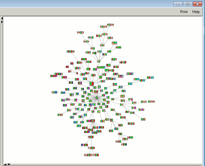
The graph panel shows the plot of related Pfam domain
architectures. The nodes of the graph dynamically jiggle about in an
effort to achieve a less cluttered layout. This optimization stops
automatically after 10 seconds and the plot is fitted to the
panel. However, the "Freeze Graph" button in the
Graph criteria panel (see below) allows you to halt the plot at any
time.

The button changes to "Plot Graph" which, when clicked, will restart
the optimization process.
You can click-and-drag any of the nodes at any time.
Each node shows a set of coloured boxes representing the sequence of
Pfam domains defining the particular architecture. Tall boxes
correspond to Pfam-A domains, whereas small boxes correspond to Pfam-B
domains. Some example nodes are shown below.
The red underlines in (c) indicate that there is structural
information in the PDB for two of the domains: one or more complete
structures for the first domain, and one or more partial or
fragmentary structures for the third.
The lines on the graph (ie the "edges" joining the nodes) show the
relationships between the architectures, based on the similarity of
their domain compositions.
The node corresponding to the architecture of the original search
sequence is slightly larger than the others and has a grey background.
|

Mouse operations for navigating about the graph
|
 |
Navigation about the plot
Navigation around the plot is as described on the left (taken from the
Graph Criteria Panel (described later).
Of these operations, the most informative is left-clicking on a node.
This provides information in the Data Panel (see below)
describing the node's constituent domains and listing the protein
sequences that have the given architecture. The data panel also
identifies which sequences, if any, have whole or partial structures
in the PDB.
Clicking the small black triangles between the panels allows you to
close/open either panel. You can also adjust the size of a panel by
left-click dragging the separator. Note that the Graph Criteria
Panel cannot be reduced beyond a certain point.
|
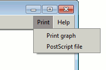
Print options menu
|
 |
Printing the graph
The Print menu at the top right-hand corner of the frame gives
you options for printing your graph.
The first option, Print graph, dumps the graph image to your
printer. This may not always produce a particularly high-quality
image.
The second option, PostScript file, writes a PostScript
file. This is scalable and so can be used to generate high-quality
prints or images, or even be converted to, say, a PDF file.
|
2. Data panel
The data panel shows the detailed information about specific nodes.
Initially the parent sequence's node is shown, as below,
together with a key to the plot and some statistics.

Click to enlarge
The statistics in red advise you that
some data has been omitted, as when the number of architectures or
protein sequences exceeds the maximum permitted. (The maximum number
of architectures allowed can be increased, as already mentioned
above).
Below the key is a list of the Pfam domains making up the parent
sequence's architecture. This gives the Pfam identifiers and the names
and descriptions of each domain. The hyperlink on the Pfam identifier
will take you to that domain's page in the Pfam database (which
should open in your web browser).
Below this list is a table listing all the domains on the plot,
in decreasing order of occurrence. The last two columns in this table
show the number of occurrences of each domain on the plot and the
number of architectures it occurs in.
Clicking the small black triangles separating the Data panel
from the Graph panel allows you to close/open either panel. You
can also left-click-drag the border between the two panels to adjust
their relative size.
Node details
If you left-click on any architecture node in the Graph panel,
the data panel will display the following information about that node:

Click to enlarge
The first table above shows the Pfam domains making up the selected
node's architecture.
The second table lists the UniProt sequences that have this domain
architecture. The table gives the UniProt ref (ie accession number),
which is hyperlinked to the appropriate page in UniProt, the
UniProt code, a marker indicating whether there are one or more 3D
structures of this protein in the PDB, the number of PDB entries, and
the protein name. Proteins with structural information in the PDB
are given priority and listed first. (Only the first 100 sequences are
listed if there are more than this number. For a full list, use the Pfam
database. Or, if you are just interested in proteins from a particular
species or only those having 3D structures, go to the Search Criteria
Panel and make the appropriate selections before generating the
plot again).
A full green tick  in the PDB column
indicates that there is at least one 3D structure in the PDB of the
full-length protein. A dashed green tick in the PDB column
indicates that there is at least one 3D structure in the PDB of the
full-length protein. A dashed green tick  indicates that, at best, the PDB contains
partial structures of the protein only. Clicking on either type of
tick will take you to a
PDBsum page listing the 3D structures that are available. indicates that, at best, the PDB contains
partial structures of the protein only. Clicking on either type of
tick will take you to a
PDBsum page listing the 3D structures that are available.
3. Graph criteria panel
 |
 |
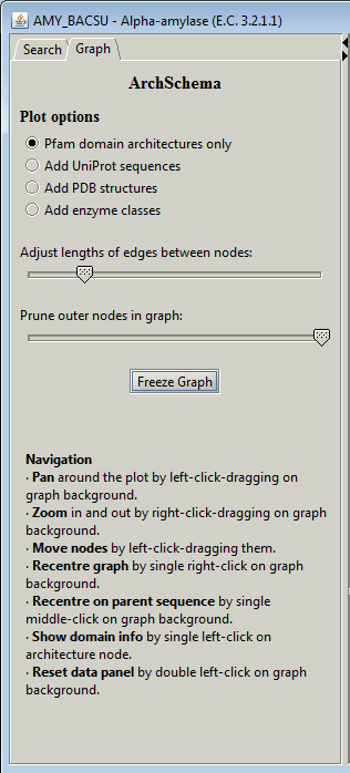
The graph criteria panel allows you to alter some of the parameters
affecting the display of the graph.
The first thing to do may be to click on the Freeze Graph
button to freeze the graph's jiggling as it strives to optimize the
relative placement of the nodes.

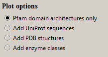
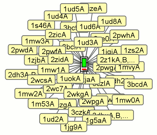
The Plot options radio buttons allow you to switch on either
the UniProt sequences belonging to each Pfam architecture, or the
PDB structures, or enzyme classifications.

These will then appear, attached to their parent nodes, as below:
 |
 |
 |
| a. UniProt sequences |
|
b. PDB structures |
 |
 |
 |
| c. Enzyme classes |
|
d. Many satellite nodes |
The nodes in example d are coloured red to indicate that
there are too many sequences to display, so only a selected number are
being shown.
Below the Plot options are two sliders. The top slider allows
you adjust the typical lengths between the nodes on the graph to get a
more compact or more distended plot.

The bottom slider is useful if you have a large graph with many
architecture nodes. It can be used to prune some of the outer nodes.

Clicking the small black triangles separating the Graph Criteria Panel
from the Graph Panel allows you to close/open either panel.
The Search tab at the top of this panel will replace it by the
Search Criteria Panel, described next.
|
Search Criteria Panel
 |
 |
The search criteria panel allows you to either initiate a new search,
or to filter the sequences returned by the current one. The latter
may be particularly useful if the initial search returns a huge number
of sequences.
The large text box lists the all domains in the current sequence. It
shows their Pfam identifiers, names and number of
sequences. Initially, all are selected. Click on any domain to select
it, and shift-click to add others to the selection.

The radio buttons above this list allow you to specify whether the
architectures to be returned should contain all the selected
domains (ie the AND option) or one or more of the
selected domains (ie the OR option).

Note that, if you select all the domains and use the AND
operator you will, of course, only get a single node on the plot:
namely, that of the parent architecture.
The Organism button lists all the species for which proteins
containing any of the above domains were found in the initial
search. Each shows the species and number of protein sequences. Select
which species to filter the sequences by.

The Sequences button allows you to limit the search to just
those proteins for which there is a complete or partial 3D structure in
the PDB.

Once you have made your selections, click on the Plot Graph
button to retrieve the data and plot the graph.

Note that, if your selection criteria happen to exclude the parent
sequence, it will still be returned by the search for reference purposes.
|
Algorithm
The graph is built by first calculating the all-against-all
similarities of all the architecture nodes. These are used in
determining which nodes to connect. The method of connecting the nodes
by edges uses a heuristic algorithm which we find gives the
intuitively best depiction of the relationships between the nodes.
Calculating the similarity of two domain architectures
Two architectures are compared by aligning their strings of domains
using the Needleman-Wunsch algorithm. Identical domains receive a
match score of 10 while non-identical domains score 0. A gap penalty
of 5 is used.
Once the alignment has been obtained, a "distance" is calculated
between the two architectures by scoring all the positions in the
alignment where the domains differ or constitute "insertions". If
either of the domains at the mismatch position is a PfamA domain, its
contribution to the distance score is 8, whereas if the mismatch
position aligns two PfamB domains the score is 4. A PfamA domain
aligned with a gap scores 4 while a PfamB domain aligned with a gap
scores 2. Any insertion within the overlap region scores an extra 1.
Any architecture that contains the parent domain architecture as an
uninterrupted substring, is scored at a distance of 3 from the
parent. This last rule ensures that architectures containing the
parent are joined to it in the graph.
Joining the architecture nodes by edges
One the all-against-all distances have been computed between the
architectures on the plot, the edges joining pairs of closely related
nodes are computed. The calculation starts with the parent node. All
architectures that are the same (minimum) distance away from it are
joined to it. Once these have been connected, the minimum distance
between all the connected nodes and those still to be connected is
calculated. All pairs of connected/unconnected nodes that are this
minimum distance apart are connected. This step is repeated until no
more unconnected nodes remain.
 |


 in the PDB column
indicates that there is at least one 3D structure in the PDB of the
full-length protein. A dashed green tick
  indicates that, at best, the PDB contains
partial structures of the protein only. Clicking on either type of
tick will take you to a
PDBsum page listing the 3D structures that are available.
