PDBeAnalysis tutorial
Introduction
This
tutorial is designed to introduce you to the PDBe analysis services of PDBeValidate,
PDBeStatistics, PDBeSelect, PDBeResidueStatistics and PDBeDatabase. These
services allow analysis of the molecular structure data (via PDBeValidate) and
also simple statistical analysis of data help on molecular structure data at
the entry and residue level.
PDBeValidate : Macromolecular structure validate
PDBeStatistics : Statistical analysis of structure
data at the structure level
PDBeSelect : Selection of macromolecular structures
PDBeResidueStatistics : Statistical analysis
of structure data at the residue level
PDBeDatabase : SQL query interface to the PDBe database
PDBeEntryResidue
: Statistical analysis of residue based data dependent on entry based data.
PDBAtomStatistics : Statistical analysis of structure data at the atom
level.
Getting started
You can access
the PDBeAnalysis services from the PDBe front page http://www.ebi.ac.uk/pdbe using the PDBeAnalysis
link within the service list. You will be presented with an intermediate jump
off page for the 5 analysis services, with an entry box for the structure ID
code for validation.
The PDBeValidate
service is designed for the analysis and presentation of information about a
single macromolecule, specifically for the identification of geometrical
outliers. PDBeStatistics, PDBeSelect and PDBeResidueStatistics are designed for
the statistical analysis of a property over all (or subset of) the PDB archive.
In fact, the analyses are based on the assembly structure of the macromolecules
and not the deposited experimental data. It is therefore hoped that these
services will provide some meaningful insight into basic analysis of macromolecular
structure. PDBeDatabase is a service that allows direct use of our database
using SQL to do select queries, so is
probably of limited use to many people.
PDBeValidate.
From the PDBeAnalysis
jump page http://www.ebi.ac.uk/pdbe-as/PDBeValidate
please enter the ID code 2sod into the entry box on this page and click
the button [validate]. This will take you to the validation page for the
protein superoxide disumutase. This structure has a reputation of being not
quite up to the normal standards of structure determination at this resolution.
The page will
open to show the view on the right. If you scroll to the bottom you will see a
quick help section that will get you started. You can see a summary table at
the top, a graph (the Ramachandran plot) 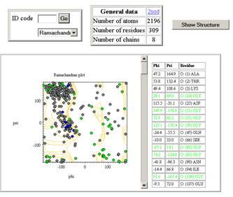 and a table of outliers. From the summary table at the
top of the view please click the 2sod
link, this will open the atlas page for this structure in a new window. You may
close this window, or hide it, it will not effect the usage of PDBeValidate. You
can see the basic detail of the structure from this page, and there are links
to view assembly, sequence, citation, similarity, ligands and visualization of
this structure. Close or hide this summary page.
and a table of outliers. From the summary table at the
top of the view please click the 2sod
link, this will open the atlas page for this structure in a new window. You may
close this window, or hide it, it will not effect the usage of PDBeValidate. You
can see the basic detail of the structure from this page, and there are links
to view assembly, sequence, citation, similarity, ligands and visualization of
this structure. Close or hide this summary page.
You will see that
the default graph is the Ramachandran plot which contains grey, blue and green
plot points. The green points are data from GLY residues and these do not have
to be within the allowed regions marked with contours. The blue points are from
PRO, and should have phi values only around –90 degrees with a variance of 12
degrees. Finally, the grey points are for all other residue types found in
proteins, and should mostly within the contoured region. As you can see there
are large numbers of outliers for this structure, and these are shown in the
table. The table is colour coded using black/green and blue data values that
match those of the graph, though there are no PRO outliers. The graph and table
are active, in that clicking points and cells results in something happening.
1) Click any
point in the graph outside a contoured region. You will see the table moves so
that the equivalent point is centred and marked in yellow. What happens if you
click a point that is within a contoured region of the graph, and why.
2) Click any cell
in the table in the third column headed residue.
You will see the equivalent point in the graph highlighted in magenta.
3) Click the
[Show structure] button at the top right, this will change to [ON] while the
AstexView@PDBe-EBI loads, and turns back to [Hide Structure] when the viewer
appears. Only the structure related commands are available in this version of
the viewer. Clicking either a graph or table value will update the structure to
highlight the picked point. Try picking a few points from the table and graph
and look at the structure. We have noted that there is a problem with the
amount of space on your screen to show the validate page and the viewer, so the
viewer is left as a floating window so you can place this somewhere sensible, though
this is not ideal.
Click the [Hide
structure] button and the viewer will close.
4) Click on the
drop down arrow next to the word [Ramachandran] in the top left control box, a
number of different validate methods will become visible. Select [omega] from
the list. This is the torsion angle CA-C-N-CA for a di-peptide and is normally
found in a trans conformation, there is one CIS conformation in this structure,
it is not a proline. Cis peptides are
usually present for a reason within a structure as they are high energy
conformations, except for proline where the cis and trans conformations are of
similar energy. Therefore, if a cis residue is not proline (marked blue on the
graph and in the table), and not near an active site then the conformation is
likely to be suspect. How would you check the positions of the active sites in
the viewer ?
5) Try a number
of different validation options and look at the analysis. What are they
attempting to show ?
6) This is a more
difficult question, though is a reminder of what you should think about when
analysing structures : Load the structure 1mbd into the validation service and
click on the [bond error] option. You will a significant number of residues
where the mean bond deviation over a residue is large, why is this ? It is a
1.4A structure so should be quite good. Hint : look at the date of release,
then think how the bond errors are calculated .
PDBeStatistics
Click on the link to PDBeStatistics from the main PDBeAnalysis page. The
service may take a second or two for the first load as the controls are
downloaded and instantiated within your browser; future visits to the page will
result in a much quicker start up. If you scroll to the bottom of the page you will
see a quick help section. When the page opens you will get an empty PDBeStatistics
page, similar to the figure on the right, but without the graph and table. This
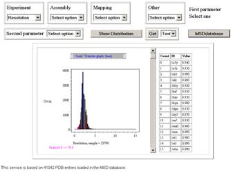 service is designed to return distributions based on a
number of data calculated from the deposited structures.
service is designed to return distributions based on a
number of data calculated from the deposited structures.
The service has 4
selection boxes along the top of the page, and then on a second line a number
of different controls.
1) The set of 4
controls at the top of the page actually control a single parameter, they have
been split into 4 to provide some clarity and also reduce the length of the
option list of a single combined set.
2) The parameter
option box on the second row of controls provides access to a second
independent residue for analysis. This control, when set to [select option]
results in only a single parameter analysis, but when an item is selected then
a 2 parameter analysis is created.
3) [Show
distribution] is the action button that draws a graph based on the options set
in (1) and (2). Clicking this button does a query against our database and
produces the graph similar to the figure above.
4) [Get] The Get
action button allows you to download either the raw data from a graph, or the
data in a table so it is available locally. The raw data for a graph
(distribution) is downloaded if no table is present, otherwise the table of
data is downloaded, and in both cases this can be obtained as text, XML, or the
SQL command to generate the data.
5) [PDBeDatabase]
action button will transfer the last query (as SQL) to the PDBeDatabase service
so that it can be adapted.
From the
[Experiement] drop down list at the top left of the page select the Resolution option, then click the [Show
Distribution] button. You will get a counter within the web page that counts up
and suggests that the query will take about 3 seconds; the timing depends on
the database load of our service, and also download time of the data which is
dependent on the bandwidth available to you. On completion of the query you
should see the graph as shown in the figure above, no table will be shown yet.
What is this graph ? Make sure you understand how this
is calculated as this is critical for the understanding.
At the top of the
graph is a double scroll bar. You may slide the two end bars independently
(with a click and drag action), or both together by click/drag of the central
region. Try this, what happens to the graph ? What happens to the Y-ordinate if
you slide to one end so the large peaks are scrolled off the view ?
Click the top of
0.9A bar from this resolution distribution. The table appears, and so your page
should look like the image above. This table contains a list of the PDB code
where the resolution is between 0.85A and 0.95A, and as of 9/11/2006 there are
91 such structures.
What happens of
you click the id code of a molecule from the table? Ie select the cell containing
1bxo, the second column, 6th row (the row may be different if new depositions
move this row). What happens if you click on the cell containing the number a,
ie the count number of the ID code 1bxo?
You can see that
the graph can make queries to our DB, and the table can open other services.
Now select
[assembly type] from the assembly options, second item on the option list in
the second drop down list, click the [Show Distribution] button. Why is this
drawn as a pie chart and not a distribution ?
Notice that you
cannot read many of the labels as they overlap, so try using the double scroll
bar to control the view. How many assembly types contain just 0.001 % of the
data and how many entries are there in one of these segments ? (Hint : click
one, what is in the table ?)
Select the
Octameric structures, this is the 6th largest segment, you may need
to slide the max slider along to view this segment easily. How many entries are
there with this assembly type ? How would you get this list as
XML ?
Can you create a
distribution of resolution as a function of R-factor ? What type of plot is
produced? Rotate the graph using a click
and drag action so that it turn flat on the screen and pull the max slider
completely to the left so it is next to the min slider. So how does R-factor
and resolution correlate?
Why is it not
possible to draw a graph of resolution as a function of assembly type?
PDBeSelect
The PDBeSelect
service is quite similar to PDBeStatistics, but allows you to combine many
different selections to create a multi-filter query against the database. When
you go to the PDBeSelect service (from the PDBeAnalysis jump page)
you should see a page 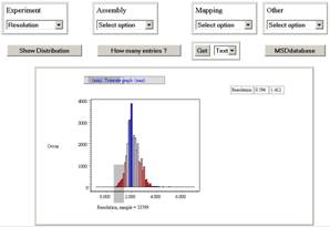 similar to that on the right without the graph and
table. The four top controls are identical to those from PDBeStatistics, and
allows the same distributions to be created. In the view on the right is the
distribution of resolution.
similar to that on the right without the graph and
table. The four top controls are identical to those from PDBeStatistics, and
allows the same distributions to be created. In the view on the right is the
distribution of resolution.
Select the top
left drop down and pick resolution. Now click the action button [Show
Distribution]. You will now see the distribution of resolution as shown in the
figure on the right (note it has been adjusted with the min-max slider
controls). The next thing it to select a range from this.
1) click a point
on the graph. You will see that an entry is put in the table of
Resolution/min/max where min and max are the same and from the column you
picked from the resolution graph.
2) click and drag
a region, ie click down at about 0.0 on the x-ordinate (resolution), and drag
the mouse to the right until you reach 2.0 on the x-axis. You will see a grey
box appear on the graph that shows you what you have selected. Now the table is
filled with Resolution/min/max where min ~ 0.0 and max ~ 2.0.
You can repeat
this selection as many times as you want, and at any time. If a resolution
entry is already present then this will be updated to the values you select,
otherwise a new entry is put in the table of your selected range.
You are now free
to select other options form the 4 drop down menus. Select the assembly type
(in Assembly) octameric by clicking
the range from the pie chart; and proteins with 2000 or less residues (from
Other). If you have a selection range you want to delete from the table you
need only click on the field column in the table of the row you want to
delete. The row will be removed from the table. How many proteins are there
with a resolution between 0 and 2A, that have an octameric assembly and have
less than 2000 residues ? Hint, what does [How many entries ?] do. Now download
the list of protein IDs as XML.
You may find this
method a little difficult to get exactly what you want, it is really a browser
of data; I have a resolution range between -0.008 and 1.932. You are now going
to fine tune this. Click on the [PDBeDatabase] button and PDBeDatabase will
open with the last query you made.
Therefore make sure the last thing you did from PDBeSelect was to click
the button [How many entries ?].
PDBeDatabase
PDBeDatabase is
used to create queries against the PDBe search schema using SQL. There are some
preset queries you can use, and if you have come to PDBeDatabase from other PDBeAnalysis
services then you will see the type of queries used to create distributions. If
you have come from the PDBeSelect section of the tutorial above then you will
see a view similar to that on the right, so please jump to this section the tutorial to work with this
query.
The PDBeDatabase
page contains a number of controls, the top left is the most simple 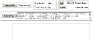 that just shows the contents of various key tables in
the database, as well as lists of tables, attributes and indexes. Click [Show
table] with the default table summary and you will get a list of all the tables
in the PDBe search database. Note that the data does not come back in any
particular order, since there is no predefined order to a database, but you can
sort the data by clicking the title bar. Notice also that there are limits to
both the number of rows you can return, and the time allowed for a query, and
both of these limits cannot be adjusted to more than 1000 and 600 respectively.
Therefore, since most of our data tables contain more than 1000 rows, you
should use filters to view the data of interest.
that just shows the contents of various key tables in
the database, as well as lists of tables, attributes and indexes. Click [Show
table] with the default table summary and you will get a list of all the tables
in the PDBe search database. Note that the data does not come back in any
particular order, since there is no predefined order to a database, but you can
sort the data by clicking the title bar. Notice also that there are limits to
both the number of rows you can return, and the time allowed for a query, and
both of these limits cannot be adjusted to more than 1000 and 600 respectively.
Therefore, since most of our data tables contain more than 1000 rows, you
should use filters to view the data of interest.
Change the table
to show to [Table column] and click show table, you will only get 200 rows back
as this is the default limits. Therefore, change the Row Limit to 1000 and try
again. What happens if you set this to
2000?
The [Get] button
allows you to download any data in the current main table. Essentially it
re-issues the last SQL used again with no row limit constraint. (The time limit
is always present). The data is returned to a new window as text or XML. Why do
you think there is a [count] button in this control box?
Try typing select something into the text box and
submit this query. You will get an oracle error returned in the table OEA-00923: FROM keyword not fou. You can see what the rest of the error is by
dragging the title divider bar to the right. All the oracle errors are returned
as a title bar in the table.
If you have come from the PDBeSelect then you will be able to modify the query
to change the resolution range to exactly between 0 and 2A. Edit the text box
so that the string reads entry.res_val
between 0 and 2; you can see that previously I had entry.res_val between –0.0080 and 1.932. (You may need to use the scroll buttons on
the right of the text entry to find the relevant piece of SQL). Click the
button [submit SQL] and the query will be run returning the table with the 158
results ( on the 7th of November 2006). The table contains the same
type of data as in PDBeSelect table for the combined filter, but in this case
the column titles are the real attribute names in the database.
PDBeResidueStatistics
The residue statistics
service allows queries to be made based on the residue data within the PDBe
search database. As of 9th/11/2006 there are 19,559,590 non-symmetry
related residues within the database and these form the basis of the queries
possible from this service.
The page
contains a number of control sets, a number of action buttons, and a graphical
area at the bottom that presents the data. Any data presented in the graph can
be obtained as raw data from the PDBeDatabase service by clicking the [PDBeDatabase]
action button. You can then re-run the SQL. The 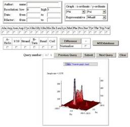 top right control set provides
structure-based filters to include/exclude different data. You can select data
based on author name, resolution, date and R-factor. The top right control box
defines the x-ordinate and y-ordinate that will be returned within a graph. The
default is 1 ordinate only of omega values. This control box also allows you to
select the representative set to use in the analysis. In general, similar
protein structures are likely to have very similar residue properties, so you
should use a representative set for any analysis you require. There is still an
option to use no representative set (NONE), but this is not recommended.
top right control set provides
structure-based filters to include/exclude different data. You can select data
based on author name, resolution, date and R-factor. The top right control box
defines the x-ordinate and y-ordinate that will be returned within a graph. The
default is 1 ordinate only of omega values. This control box also allows you to
select the representative set to use in the analysis. In general, similar
protein structures are likely to have very similar residue properties, so you
should use a representative set for any analysis you require. There is still an
option to use no representative set (NONE), but this is not recommended.
The
control box on the second row allows an analysis to be made for 1 or more
residue types. If none are selected, then all residue types are used in the
analysis. The third row contains a control box that limits the secondary
structure type for the residues in the analysis, if none is selected then all
structure types are included.
The [PDBeDatabase]
control button will drop the SQL used to create a graph into PDBeDatabase to
allow modification, or get the raw data.
There are
a number of different control buttons, [submit] is the good first starting
point, in fact just click submit with all the controls as they are set. You will get a distribution of omega for all residues in the Dali
representative set. This will take about 1 minute to calculate. We are now
going to do something a little more interesting, find how the 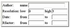 Ramachandran plot changes with
resolution.
Ramachandran plot changes with
resolution.
Within
the top left filter box, set the resolution range between 0A and 1A range as
shown on the left.
 Now change the ordinate selection so that phi is the
x-ordinate and the y-ordinate is set to phi; this is this Ramachandran graph
ordinates. I have selected the WhatIf representative set here.
Now change the ordinate selection so that phi is the
x-ordinate and the y-ordinate is set to phi; this is this Ramachandran graph
ordinates. I have selected the WhatIf representative set here.
Now click the
[submit] button. You will get 2D distribution of phi against psi with a sample
size a little under 16,000 data for this high resolution set; quite similar to
the graph at the top of this section. Now go back to the resolution range boxes
and change the range to low=2A and high=3A. This query will take longer as
there are many more data in this resolution range, and a similar graph will
appear with a sample size of about 1 million.
You can see that
the service has remembered you old queries, and the main control line shows
which query number you are on, the first query was the simple omega query, the
second query was the high resolution phi/psi and the third was the lower
resolution phi/psi, giving a total of 3 queries, and you are looking at query
number 3. Click the [Previous Query] button and the page will show the high
resolution query, and clicking this again will show the omega query. Notice how
all the form fields are updated to reflect the query, not just the resulting
graph.
Now we what to
calculate a difference plot for high and low resolution Ramachandran data. Make
sure the last 2 queries are the low and high resolution 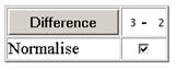 phi/psi search, you can use the previous and next control
buttons to check this. Now look at the page to find the difference control box,
and select the normalise check box as
shown on the right; click the [Difference] control button. You should get a
difference plot for the phi and psi ordinates for the two resolution ranges.
phi/psi search, you can use the previous and next control
buttons to check this. Now look at the page to find the difference control box,
and select the normalise check box as
shown on the right; click the [Difference] control button. You should get a
difference plot for the phi and psi ordinates for the two resolution ranges.
1) What did the
normalise check box do? Do a difference plot without the normalise option
checked to see the difference.
2) In the
difference plot, what does the sample size measure? (see the graph title).
3) Use the min
and max scroll bars to zoom in on the zero z-ordinate, and turn the plot so it
looks like a contour plot, what do you see in the alpha helix region?
3) Now create a
difference plot of Ramachandran for ASN and ASP, what do you see when you zoom
in to highlight the near zero z-ordinate ?
4) What happens
if you pick a point on the graph, what do you think is returned ?
PDBeAtomStatistics
PDBeAatomStatistics
is used to look at atomic data based on 1-2 interactions (bonds and
non-bonding), 1-3 interactions (angles) and 1-4 interactions (torsion angles). The
service is based on the 0.5 billion atom data rows within the PDBe database. It
is possible to generate some long queries here, but the default set of filters
provided will generally return results in about 30seconds to 1 minute.
 Note, that due to restrictions of data return size it
is possible to do queries that return a truncated list of results. This is to
protect the client and server side resources from large volumes of data. In
general you will not improve statistics by selecting filters that would return
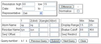
huge quantities of data. The PDBeAtomStatistics interface is shown in the
figures and it is clear that this service is more complicated that all the
other statistical interfaces and allows a number of different possible queries.
It has filters based on entry data (resolution, date and representative set) as
well as up to 4 atom definitions with sequence dependences. The main query box
contains 11 field boxes for Atom Name, Residue Name and sequence Offset. Atom
name is the standard atomic name, and to the left is shown SG, the gamma
sulphur atom for cystine. In the example query only 2 atom names are given
which means the query will return distance
Note, that due to restrictions of data return size it
is possible to do queries that return a truncated list of results. This is to
protect the client and server side resources from large volumes of data. In
general you will not improve statistics by selecting filters that would return
huge quantities of data. The PDBeAtomStatistics interface is shown in the
figures and it is clear that this service is more complicated that all the
other statistical interfaces and allows a number of different possible queries.
It has filters based on entry data (resolution, date and representative set) as
well as up to 4 atom definitions with sequence dependences. The main query box
contains 11 field boxes for Atom Name, Residue Name and sequence Offset. Atom
name is the standard atomic name, and to the left is shown SG, the gamma
sulphur atom for cystine. In the example query only 2 atom names are given
which means the query will return distance 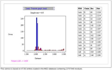 information. Residue name information is optional, and
in the example shows the residue cystine. It is also possible to supply a comma
separated list of residues within a box to indicate an atom can be any of the
supplied residue list (eg. asp,glu), though in this example SG is only found in
cystine so this would not be relevant. Finally, the sequence offset is useful
for more general interaction specifications. If we consider the disulphide bond
example we would not normally provide any sequence offset requirement since the
2 atoms within a disulphide do not have a specific sequence dependence; though
see later for a sequence restrictions which may be of use. The sequence offset
box is therefore left clear in this example. If we consider the query to look
for the backbone torsion angle omega within proteins then we
information. Residue name information is optional, and
in the example shows the residue cystine. It is also possible to supply a comma
separated list of residues within a box to indicate an atom can be any of the
supplied residue list (eg. asp,glu), though in this example SG is only found in
cystine so this would not be relevant. Finally, the sequence offset is useful
for more general interaction specifications. If we consider the disulphide bond
example we would not normally provide any sequence offset requirement since the
2 atoms within a disulphide do not have a specific sequence dependence; though
see later for a sequence restrictions which may be of use. The sequence offset
box is therefore left clear in this example. If we consider the query to look
for the backbone torsion angle omega within proteins then we 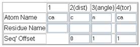 can use the query design shown. The atom names are
defined as (ca-c-n-ca), there is no residue specification since we want to look
at all possible residues, and the sequence offset has been filled in with the
values (0-1-1) where the first atom has an assumed value of 0. If we re-write
the definition of the omega torsion as a function of the ith residue
then we obtain ca[i+0]-c[i+0]-n[i+1]-ca[i+1] and it becomes clear that the
sequence offset in this case is the value added to I to define which residue we
are talking about relative to residue I. Notice that the first atom is always
defined as belonging to residue I. The residue names can take a number of
values; so far we have used CYS for the disulphide search and blank for a
general search. A residue value can also be a comma separated list of residues
(eg: asp,glu,asn,gln) or NOT a residue or list of residues (eg: !pro)
can use the query design shown. The atom names are
defined as (ca-c-n-ca), there is no residue specification since we want to look
at all possible residues, and the sequence offset has been filled in with the
values (0-1-1) where the first atom has an assumed value of 0. If we re-write
the definition of the omega torsion as a function of the ith residue
then we obtain ca[i+0]-c[i+0]-n[i+1]-ca[i+1] and it becomes clear that the
sequence offset in this case is the value added to I to define which residue we
are talking about relative to residue I. Notice that the first atom is always
defined as belonging to residue I. The residue names can take a number of
values; so far we have used CYS for the disulphide search and blank for a
general search. A residue value can also be a comma separated list of residues
(eg: asp,glu,asn,gln) or NOT a residue or list of residues (eg: !pro)
In general, 1-2
interactions which are bonded require a sequence offset specification while
non-bonded atom interactions (though space) have no sequence dependence and
should have no value for sequence offset included. Angles and torsion normally
require sequence offset values to return meaningful results.
The next
parameter set has 6 fields as 3 sets of min-max pair values. Distance cutoff
defines the plotted range of values that recorded for a query. Notice that
distances often require valued of 0 for min and < 10 for the maximum value;
whereas torsion and angle queries require values of 0 to 180 and -180 to 180
respectively. This is a common error when making a angle query and nothing
appears to be returned. The B-value cutoff is set to a default of min=0.0 and
max = 40.0 A2 where the B-value defines the refined 4th
atomic parameter within crystallography and how well locallised that atom is
and how well observed. If you unclear about the meaning of B-value then it is
recommended you leave the values at the default. The final filter pair is
sequence restriction. These number (with no default value) are only of use for
through space 1-2 interactions, ie non-bonding or disulphides, where the values
define the minimum and maximum sequence distance between the atoms in the query.
1) Perform an
Omega torsion angle query. Fill in the atom definition first; what do you
notice about the min and max values as you add the 3rd and 4th
atom definition ?
2) How would you
create a search for omega where the residue i+1 is proline only, and then NOT
proline.
Finally, the
difference function block. The difference function allows the presentation of
results as the numerical difference (either normalised or not) between the
current result and the last result. Since all the analysis returns 72 bin
distributions it is possible to calculate a difference function between any 2
result sets, so it is up to the user to actually make a sensible judgement of
whether a difference function is meaningful. The normalise option within the
difference block is used to equate the areas under the curves before
subtraction so data can be compared even where the number of results is not
equivalent.
3) Calculate a
difference function for omega for residues when (i+1 = PRO) and then (i+1 =
!PRO).
4) What do you
notice about the cis/trans distribution; did you expect this ?
There are action
button to run a query, look at the previous and next query in the list as well
as clear the fields to the default values. A query will be shown as running by
a counter in the graph window, and the graph can be picked to return a selected
list of atoms in a table. The table of atoms can be picked to either open the
atlas page for the entry containing the atom (selecting the PDB-ID), or open PDBeValidate
(with optional link to the AstexViewer@PDBe-EBI structure viewer).
5) You might like
to see how omega varies as function of resolution (0 to 1.5A range and 2.0 to
2.5A).
Data saturation
The PDBeAtomStatistics
service has an issue regarding the implementation of the service. Due to the
size of the atom data (0.5 billion rows of data) a compromise was made
regarding the service due to technical reasons. This means that any one query
many not return more than 10,000 rows, and data is correlated and extracted
from this subset of hits to give a distribution. Therefore, increasing the
return size (by increasing the resolution range) will not improve the
statistics of the results, just make the query longer. A solution to this
limitation is being sought.